POD Analysis of Turbulent Pipe Flow

M. Raba

Created: 2025-10-06 Mon 04:24

Background and Motivation

Literature Review

Background and Motivation

Talk Title: POD Analysis of Turbulent Pipe Flow

Why Rotating Pipe Flow?

Simple geometry, yet rich in turbulent dynamics
Ideal for studying rotation-induced turbulence suppression
Relevant to aerospace, combustion, and industrial flows

Historical Observations:

Rotation reduces skin friction and pressure loss
Experiments (e.g., White 1964, Kikuyama et al. 1983) showed relaminarization at high rotation rates

Research Gaps & Objectives

Challenges:

Limited DNS studies at moderate-to-high Reynolds numbers
RANS/LES models struggle to capture suppression mechanisms

Goals of This Work:

Use DNS to quantify turbulence suppression
Apply POD to identify dominant coherent structures
Provide benchmark data for turbulence model validation

This study bridges the gap between high-fidelity simulations and reduced-order modeling of rotating turbulent flows.

DNS Turbulent Model

DNS Configuration: Rotating Turbulent Pipe Flow

Flow Type: Axially rotating turbulent pipe flow

Solver: Nek5000 (Spectral Element Method)

Reynolds Numbers: 5,300 and 11,700

Rotation Numbers (N): 0 to 3

Domain: Streamwise extent of 15D, periodic boundaries

Purpose: Study turbulence suppression and provide DNS benchmark data

Numerical & Grid Details

Time Integration:

Viscous terms: BDF3 (implicit)
Nonlinear terms: Explicit extrapolation (3rd order)

Grid Resolution (wall units y⁺):

Radial: 0.14–4.4 (Re = 5300), 0.16–4.7 (Re = 11,700)
Azimuthal: 1.5–5.0
Streamwise: 3.0–9.9

Mesh: Hexahedral elements with high-order tensor polynomials

Parallelization: MPI with auto-tuned algorithms

Pressure Solver: Algebraic Multigrid (AMG)

Temporal Averaging: Over 6.5 flow-throughs (after transient)

Background: Rotating Pipe Flow & Relaminarization

Scientific Context

Rotating pipe flow is a canonical system for studying flow stabilization and relaminarization.
Rotation modifies turbulence production and redistributes momentum through Coriolis and centrifugal effects.
Relaminarization occurs when rotation suppresses the near-wall turbulence regeneration cycle.

Key Phenomena

Competition between destabilizing wall shear and stabilizing radial pressure gradients.
Reduction in Reynolds stresses and near-wall streaks at high rotation rates.
Relaminarized or quasi-laminar states can persist at high Reynolds numbers.

[1] White (1964), J. Fluid Mech. — early rotating pipe experiments. [2] Kikuyama et al. (1983), JSME Int. J. — visualization of relaminarization. [3] Imao (1996), Exp. Fluids — centrifugal stabilization and mean profiles.

DNS, Theory, and Modal Decomposition

DNS and Analytical Foundations

DNS captures relaminarization at Re = 10⁴–10⁵ under rotation.
Scaling and symmetry analyses (Oberlack, 1999; 2001) relate turbulence structure to invariants.
Hellström et al. (2017) provide reproducible experimental and DNS methodology for relaminarization.

Modal Analysis (POD)

Proper Orthogonal Decomposition (POD) identifies energy-dominant coherent structures.
Developed by Lumley (1967); extended by Taira et al. (2017) for complex turbulent systems.
Recent studies (Brehm 2019; Ashton 2019) combine DNS and POD for energy transfer diagnostics.

[1] Orlandi & Fatica (1997), J. Fluid Mech. — first DNS of rotating pipe turbulence. [2] Feiz & Tavoularis (2005), Phys. Fluids — DNS of turbulent pipe under rotation. [3] Hellström et al. (2017), Phys. Rev. Fluids — experimental/DNS methodology for relaminarization. [4] Oberlack (1999; 2001), J. Fluid Mech. — scaling and symmetry theory. [5] Lumley (1967), Atmos. Turbulence; Taira et al. (2017), AIAA J.

Control & Transition Mechanisms

Mechanistic Understanding

Rotation alters the balance of production and dissipation terms in the turbulent kinetic energy budget.
Flow control studies show relaminarization through imposed swirl or wall rotation.
Experimental relaminarization occurs by suppression of near-wall vortices and streak breakdown.

Recent Advances

Kühnen et al. (2014, 2018) demonstrated full relaminarization through wall rotation and suction control.
These results motivate DNS-based exploration of transient energy transfer and POD modal evolution.
Ongoing studies bridge classical rotation control and modern data-driven modal analysis.

[1] Kühnen et al. (2014; 2018), Nat. Phys. — experimental control and relaminarization. [2] Brehm (2019); Ashton (2019) — POD analysis of relaminarizing turbulence. [3] Kolmogorov (1941), Dokl. Akad. Nauk SSSR — statistical theory foundation.

Method Spectral Element Direct Numerical Simulation (DNS)

Slide 1: Introduction

Background

Transition and relaminarization in rotating pipe flows depend on rotation rate and Reynolds number.
Relaminarization can occur when imposed swirl suppresses near-wall turbulence production.
Applications: rotating heat exchangers, turbomachinery, compact fluid systems.

Governing Equations

\begin{align} \nabla \cdot \mathbf{u} &= 0, \\ \frac{\partial \mathbf{u}}{\partial t} + (\mathbf{u}\cdot\nabla)\mathbf{u} &= -\frac{1}{\rho}\nabla p + \nu \nabla^2 \mathbf{u} - 2 \boldsymbol{\Omega}\times\mathbf{u} \end{align}

References: Alfredsson & Persson (1989)[1], Johnston et al. (1972)[2]

Slide 2: Spectral Element Method (DNS)

Simulation Setup

Circular pipe: D=1, L=12D
Re = 5300, 12700, non-slip wall
Legendre basis, polynomial order 6
Non-uniform mesh finer near wall to capture Kolmogorov/Taylor scales

Navier-Stokes in Cylindrical Coordinates

\begin{align} \frac{\partial w}{\partial t} + w \frac{\partial w}{\partial r} + \frac{v}{r} \frac{\partial w}{\partial \theta} + u \frac{\partial w}{\partial x} - \frac{v^2}{r} &= -\frac{1}{\rho} \frac{\partial p}{\partial r} + \nu \left(\mathcal{D} w - \frac{w}{r^2} - \frac{2}{r^2}\frac{\partial v}{\partial \theta} \right) - 2\Omega v \\ \frac{\partial v}{\partial t} + w \frac{\partial v}{\partial r} + \frac{vw}{r} + \frac{v}{r} \frac{\partial v}{\partial \theta} + u \frac{\partial v}{\partial x} &= -\frac{1}{\rho r} \frac{\partial p}{\partial \theta} + \nu \left(\mathcal{D} v - \frac{v}{r^2} + \frac{2}{r^2}\frac{\partial w}{\partial \theta} \right) + 2\Omega w \\ \frac{\partial u}{\partial t} + w \frac{\partial u}{\partial r} + \frac{v}{r} \frac{\partial u}{\partial \theta} + u \frac{\partial u}{\partial x} &= -\frac{1}{\rho} \frac{\partial p}{\partial x} + \nu \mathcal{D} u \end{align}

References: Kundu (2015)[3], Hellström et al. (2017)[4]

Slide 3: Mesh and Simulation Details

Mesh Details

Non-uniform grid denser near walls
Grid spacings (y+) for streamwise extent of 15D
Example: Re=5300, Δr⁺=0.14–4, Δθ⁺=1.5–4.5, Δz⁺=3–9.9

Boundary Conditions

\begin{align} u_r(R) &= 0, \\ u_\theta(R) &= \Omega R, \\ u_x(R) &= 0 \end{align}

Rotation vector: Ω = Ω e_k; smooth wall, incompressible flow

[1] Alfredsson & Persson, 1989.
[2] Johnston et al., 1972.
[3] Kundu, 2015, Fluid Mechanics.
[4] Hellström et al., 2017, J. Fluid Mech. 829:164–188.

DNS Mesh

Simulation Domain

Circular pipe, D = 1, L = 12D
Reynolds numbers: 5300, 12700
Non-slip at walls, periodic at inlet/outlet
Spectral element method: Legendre basis, order l = 6

Governing Equations

\begin{align} \nabla \cdot \boldsymbol{u} &= 0 \\ \frac{\partial \boldsymbol{u}}{\partial t}+ (\boldsymbol{u}\cdot\nabla)\boldsymbol{u} &= -\nabla p + \frac{1}{Re} \nabla^2 \boldsymbol{u} \end{align}

Mesh Images

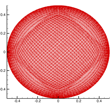
Non-uniform mesh (finer near walls)

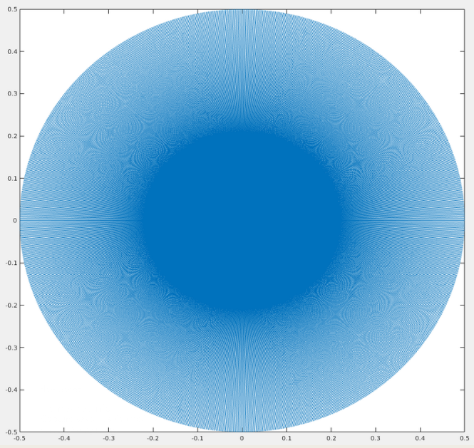
Uniform, interpolated mesh for POD analysis

Grid Spacing and Boundary Conditions

Grid Spacings (y⁺ units)

Re	Δr⁺ / Δθ⁺ / Δz⁺	N Δt × 10⁶
5,300	0.14–4 / 1.5–4.5 / 3–9.9	20
11,700	0.15–4.5 / 1.5–4.8 / 3–10	120

Boundary Conditions

\begin{align} u_r(R) &= 0, \\ u_\theta(R) &= \Omega R, \\ u_x(R) &= 0 \end{align}

Rotation vector: Ω = Ω e_k; smooth wall; incompressible flow

Proper Orthogonal Decomposition

POD Energy Modes

Direct POD Formulation

(2.1) Radial eigenvalue problem:

$$ \int S(k, m; r, r') \, \Phi_n(k, m; r') \, r' \, dr' = \lambda_n(k, m) \, \Phi_n(k, m; r) $$

(2.2) Cross-correlation tensor:

$$ S(k, m; r, r') = \lim_{\tau \to \infty} \frac{1}{\tau} \int_0^\tau \mathbf{u}(k, m; r, t) \, \mathbf{u}^*(k, m; r', t) \, dt $$

(2.3) POD coefficient projection:

$$ \alpha_n(k, m; t) = \int \mathbf{u}(k, m; r, t) \, \Phi_n^*(k, m; r) \, r \, dr $$

Snapshot POD & Conditional Mode

(2.4) Time-domain eigenvalue problem:

$$ \int R(k, m; t, t') \, \alpha_n(k, m; t') \, dt' = \lambda_n(k, m) \, \alpha_n(k, m; t) $$

(2.5) Mode reconstruction:

$$ \int \mathbf{u}^T(k, m; r, t) \, \alpha_n^*(k, m; t) \, dt = \Phi_n^T(k, m; r) \, \lambda_n(k, m) $$

(2.6) Conditional mode definition:

$$ \Psi_n(m; \xi, r) = \lim_{\chi \to \infty} \frac{1}{\chi} \int_0^\chi \int_0^\tau \mathbf{u}^T(m; r, x+\xi, t) \, \alpha_n(m; x, t) \, dt \, dx $$

FFT / POD Interpretation

FFT Decomposition in Pipe Flow

Azimuthal FFT:

Exploits rotational symmetry of the pipe
Azimuthal mode number m defines spanwise length scale
Highlights circumferential structure and periodicity

Streamwise FFT:

Captures axial periodicity and wavelength
Mode number k relates to streamwise extent of structures
Useful for identifying repeating patterns like VLSMs

Why FFT?

Geometry-driven decomposition
Modes are known a priori due to symmetry
Accelerates POD convergence

Proper Orthogonal Decomposition (POD)

Nature of POD Modes:

Data-driven: extracted from simulation or experiment
Ranked by energy content (most energetic first)
Capture coherent structures across scales

Snapshot POD:

Assumes separability of space and time
Reduces computational cost by working in time domain
Enables modal analysis of large datasets

Complementarity:

FFT modes reflect geometry
POD modes reflect physics and energy distribution
Combined FFT-POD approach enhances interpretability

Proper Orthogonal Decomposition (POD)

POD Overview

Decomposes turbulent velocity field to a reduced order model (ROM)
Orthogonal basis captures dominant flow patterns ¹
Snapshot POD faster convergence than classical POD
Hybrid FFT-POD: Fourier modes in θ, POD in radial direction

Snapshot POD: Hilbert Space

$$\langle q_1, q_2 \rangle_{r,t} = \int q_1 q_2^* r \, dr \, dt$$ $$\lambda = \frac{ E\{ | q(r,t) , \Phi(r,t) |^2 \} }{ \langle \Phi(r,t), \Phi(r,t) \rangle_{r,t} }$$ $$\int R(t,t') \Phi(t')\,dt = \lambda \Phi(t)$$

[1] Lumley, 1967; [2] Taira et al., 2017.

Snapshot POD: Eigenvalue Problem

Direct POD Equation

$$\int_{r'} \mathbf{S}(k; m; r, r') \Phi^{(n)}(k; m; r') r' dr' = \lambda^{(n)}(k;m) \Phi^{(n)}(k; m; r)$$ $$\mathbf{S}(k; m; r, r') = \lim_{\tau \to \infty} \frac{1}{\tau} \int_0^\tau \mathbf{u}(k; m; r, t) \mathbf{u}^*(k; m; r', t) dt$$

Temporal Coefficients

$$\alpha^{(n)}(k; m; t) = \int_r \mathbf{u}(k; m; r, t) \Phi^{(n)^*}(k; m; r) r dr$$ $$\lim_{\tau \to \infty} \frac{1}{\tau} \int_0^\tau \mathbf{u}_T(k; m; r, t) \alpha^{(n)^*}(k; m; t) dt = \Phi_T^{(n)}(k; m; r) \lambda^{(n)}(k;m)$$

[1] Lumley, 1967; [2] Taira et al., 2017; [3] Tutkun & George, 2001; [4] Hellström & Smits, 2014.

Classical POD Form

Correlation Tensor

$$\int_{r'} \mathbf{S}(k; m; r, r') \Phi^{(n)}(k; m; r') r' dr' = \lambda^{(n)}(k; m) \Phi^{(n)}(k; m; r)$$ $$\int_{r'} W_{i,j}(r,r') \hat{\phi}_j^{*(n)}(r') dr' = \hat{\lambda}^{(n)}(m;f) \hat{\phi}_i^{(n)}(r,m;f)$$

Time Coefficient

$$\lim_{\tau \to \infty} \frac{1}{\tau} \int_0^\tau (r^{1/2} \mathbf{u}(m;r,t), r^{1/2}\mathbf{u}(m;r,t')) \alpha_n(m;t') dt' = \lambda_n(m) \alpha_n(m;t)$$ $$\alpha_n(m;t) = \int_r \mathbf{u}(m;r,t) r^{1/2} \Phi_n^*(m;r) dr$$

[1] Tutkun & George, 2001; [2] Hellström & Smits, 2014.

Radial Projections

POD Mode Behavior at N = 0

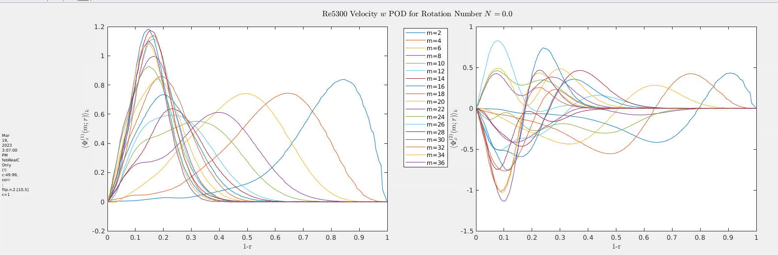
POD Mode Behavior at N = 0

Rotation Number: N = 0 (non-rotating pipe)
Flow Regime: Classical turbulent pipe flow
Azimuthal Modes: m = 2 to 36
Radial Profiles: Symmetric, peak away from wall
Conditional Modes: Show coherent structures aligned with streamwise direction
Interpretation: Near-wall turbulence is strong; structures are well-developed and span the pipe radius

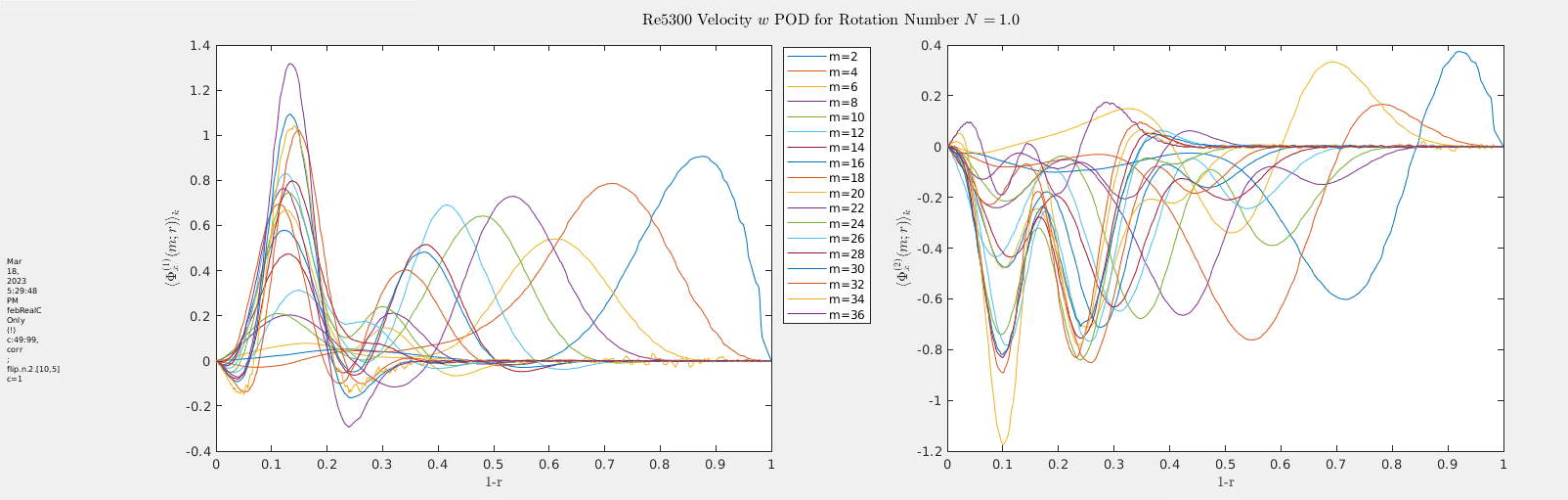
This baseline case helps contrast the effects of rotation on POD mode shape and energy distribution.

POD Mode Behavior at N = 1

POD Mode Behavior at N = 1

Rotation Number: N = 1 (moderate rotation)
Swirl Number: Ratio of azimuthal to axial momentum flux; quantifies rotational intensity
Flow Regime: Transitional toward relaminarization
Azimuthal Modes: m = 2 to 36
Radial Profiles: Begin to shift inward; near-wall peaks flatten
Azimuthal Structure: Enhanced swirl due to Coriolis effects
Interpretation: Rotation suppresses near-wall turbulence and redistributes energy toward the core

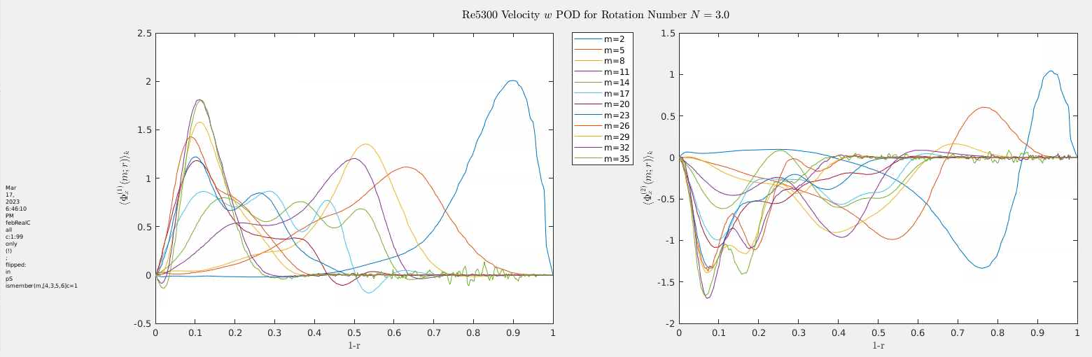
Compared to N = 0, the POD modes at N = 1 show early signs of turbulence suppression and structural reorganization.

N=3

POD Mode Behavior at N = 3

Rotation Number: N = 3 (strong rotation)
Swirl Number: High azimuthal momentum; dominant rotational effects
Flow Regime: Strong turbulence suppression; approaching relaminarization
Azimuthal Modes: Energy concentrated in low modes (m = 5–20)
Radial Profiles: Streamwise structures shift closer to wall; radial structures broaden
Azimuthal Structure: Reduced wall-normal extent; secondary peaks emerge
Interpretation: Rotation reorganizes turbulence, suppresses near-wall activity, and enhances core coherence

At N = 3, POD modes show strong coherence and redistribution of energy, with dominant structures moving toward the wall and secondary peaks forming near the centerline.

FFT-POD Mode Shapes

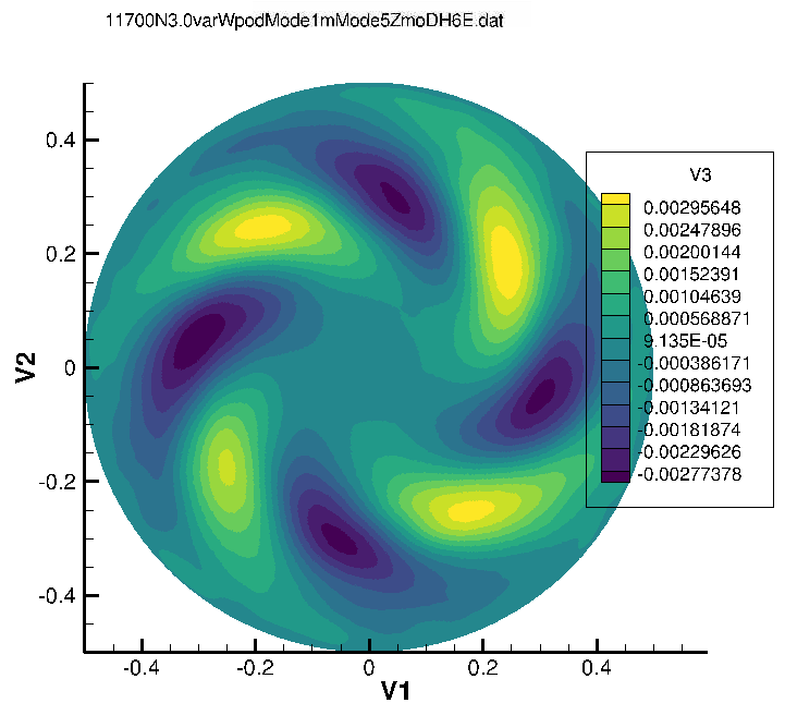
POD Mode 1 at Re = 11,700 for Azimuthal Modes m = 5 and m = 10

Azimuthal Mode m = 5 (N = 3)
Coherent structure with 5-lobed symmetry; strong modal energy concentration.

Azimuthal Mode m = 10 (N = 1)
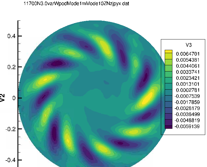
Finer-scale oscillatory structure; reduced energy per mode compared to m = 5.

Radial POD Modes

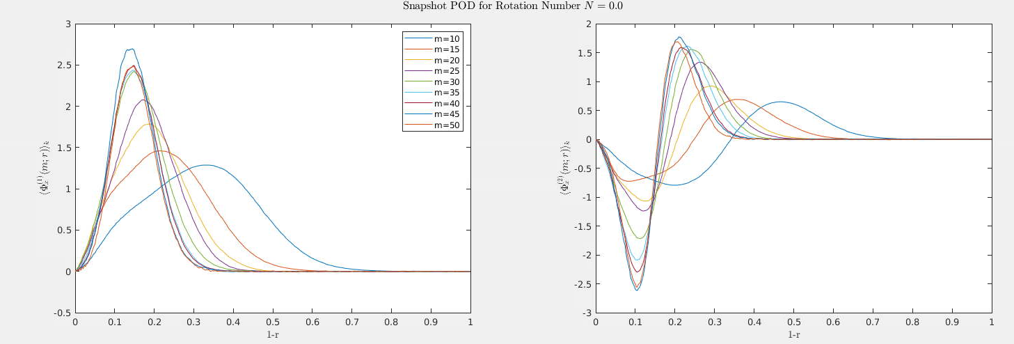
Figure 1: $N=0.0$ Radial POD Azimuthal Modes

$N=0.5$

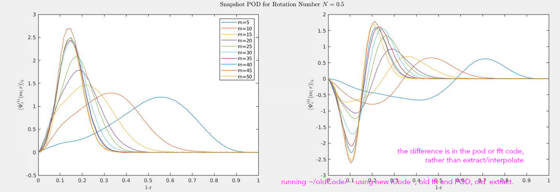
Figure 2: $N=0.5$ Radial POD Azimuthal Modes

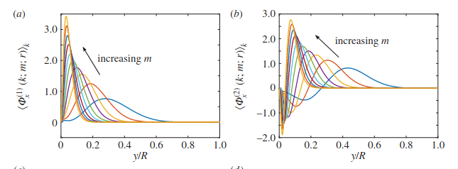
Figure 3: Ref (Hellstrom 2017 Benchmark)

$N=3$

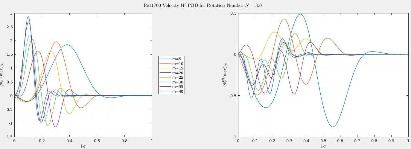
Figure 4: $N=3$ Radial POD Azimuthal Modes

Rotating Pipe POD Results

Rotating Pipe POD Results — POD Theory & 2D Projection

POD Modes & 2D Projection

Azimuthal modes m ∈ [1,30]
Streamwise-invariant, averaged along x
Phase-flipped to ensure consistent ±1 orientation
FFT in θ direction for radial profiles

Radial Modal Profile Equation

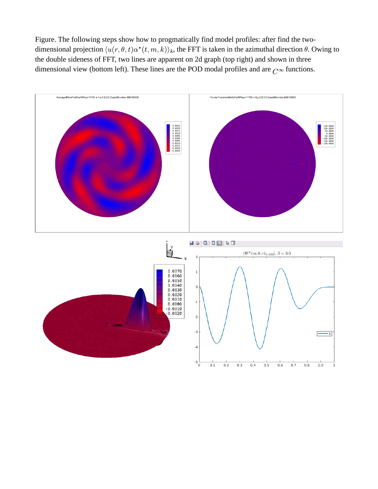
\[ \begin{align} \Phi_{\mathrm{T}}^{(n)}(k ; m ; r) \lambda^{(n)}( m) &= \left\langle\lim _{\tau \rightarrow \infty} \frac{1}{\tau} \int_0^\tau \mathbf{u}_{\mathrm{T}}(k ; m ; r, t) \alpha^{(n)^*}(k ; m ; t) dt \right\rangle \\ &= \mathcal{F}_\theta \left( \lim _{\tau \rightarrow \infty} \frac{1}{N} \sum_k^{N} \frac{1}{\tau} \int_0^\tau \mathbf{u}_{\mathrm{T}}(k ; \theta ; r, t) \alpha^{(n)^*}(k ; m ; t) dt \right) \\ &= \text{(Fourier transform in azimuthal direction of phase-shifted eigenface)} \end{align} \]

2D POD Projection Example

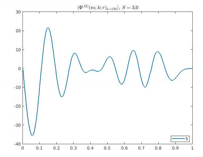
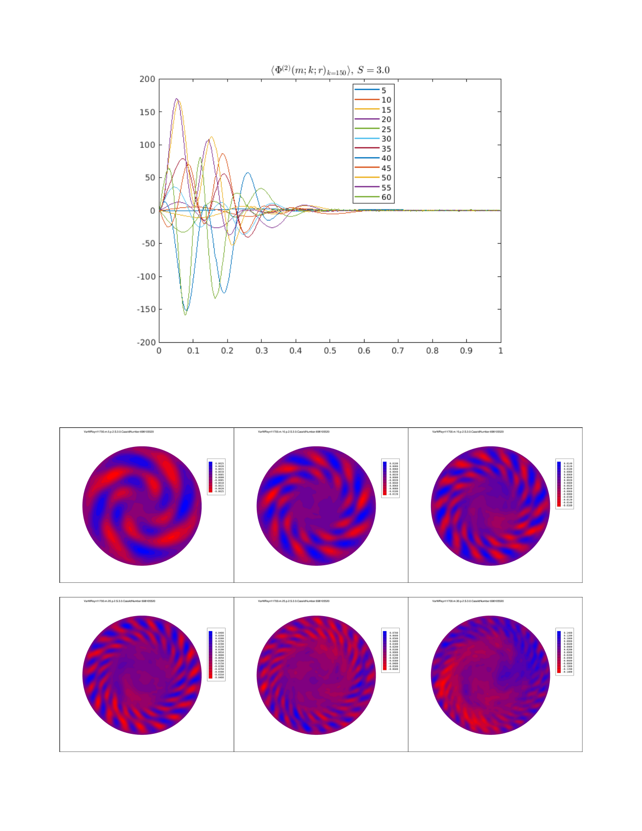
Modal Profile φ²

Streamwise Component φ², S=3.0

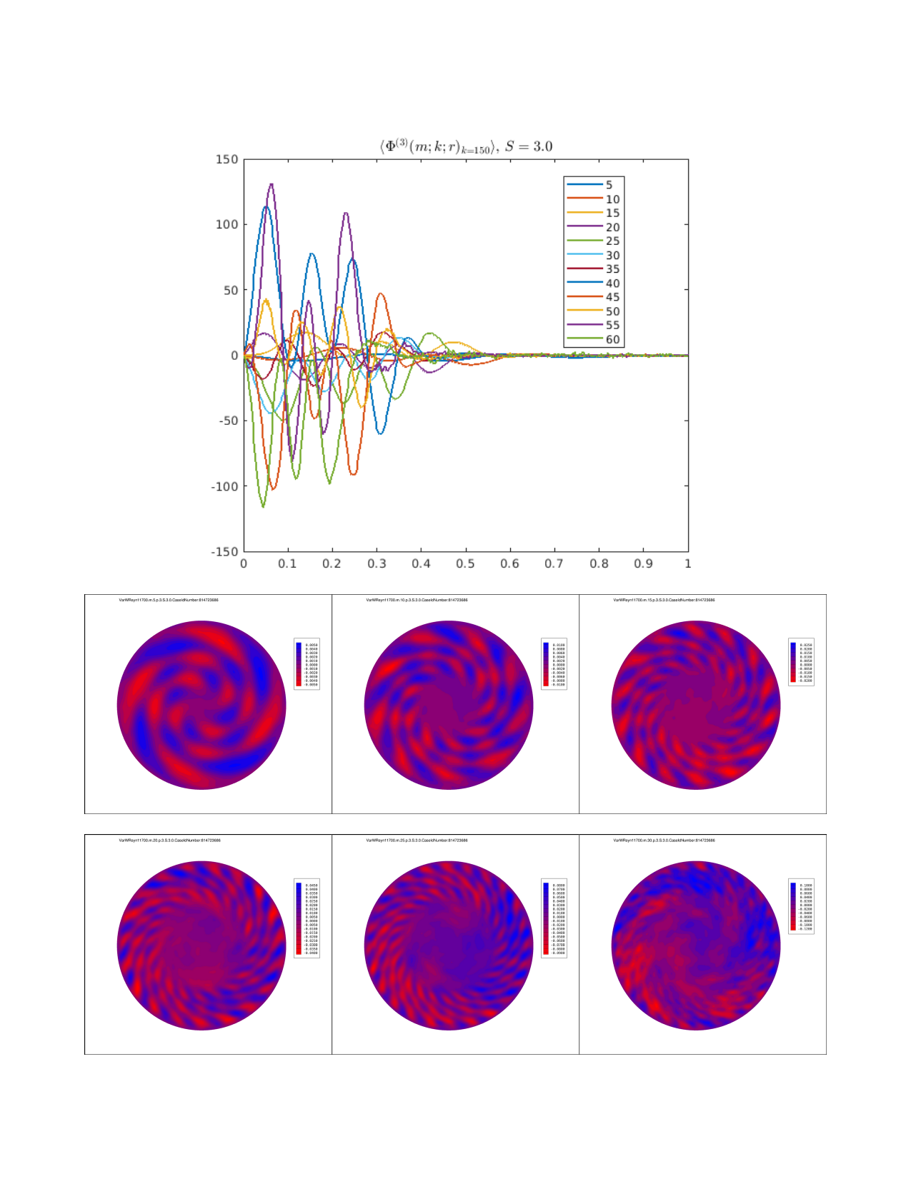
Modal Profile φ³

Streamwise Component φ³, S=3.0

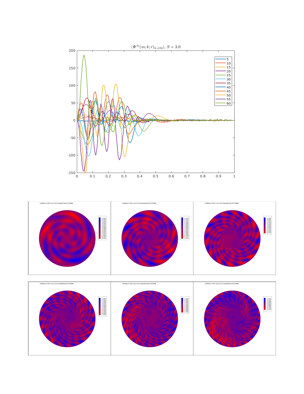
Modal Profile φ⁴

Streamwise Component φ⁴, S=3.0

Derivation of POD

Derivation of POD Projections

Citations

References

Hellström, L. H. O. (2017). Relaminarisation of Turbulent Pipe Flow through Oscillatory Forcing. PhD thesis, Princeton University
— Methodology and experimental setup for relaminarization in rotating/oscillatory conditions.
Kühnen, J., Holtz, E., Hof, B. (2014). Experimental investigation of turbulent drag reduction by wall rotation. J. Fluid Mech., 738:463–487.
— Shows streamwise wall rotation can trigger relaminarization.
Kühnen, J., Song, B., Scarselli, D., Budanur, N. B., Riedl, M., Willis, A. P., Hof, B. (2018). Destabilizing turbulence in pipe flow. Nature Phys., 14(4):386–390.
— Demonstrated full relaminarization via body forcing.
Xiao, Y., Peixinho, J. (2019). Experimental investigation of relaminarisation of turbulent flow in a rotating pipe. J. Fluid Mech., 862: R1.
— Full relaminarization achieved through global rotation.
Czarske, J., Büttner, L., Budinger, M., et al. (2002). Velocity measurements in rotating turbulent pipe flow. Exp. Fluids, 33(1):115–123.
— Laser-Doppler data showing turbulence structure changes under rotation.

Johnston, J. P., Halleen, R. M., Lezius, D. K. (1972). Effects of spanwise rotation on the structure of two-dimensional fully developed turbulent channel flow. J. Fluid Mech., 56(3):533–557.
— Classic rotation-induced turbulence suppression study.
Grundestam, O., Wallin, S., Johansson, A. V. (2008). Direct numerical simulations of rotating turbulent pipe flow. J. Fluid Mech., 598:177–199.
— DNS showing relaminarization trends with rotation rate.
Facciolo, L., Peixinho, J. (2018). Dynamics of laminar and turbulent flows in rotating pipes. Phys. Rev. Fluids, 3:034603.
— Defines critical rotation numbers for relaminarization.
Reynolds, O. (1883). An experimental investigation of the circumstances which determine whether the motion of water shall be direct or sinuous. Phil. Trans. R. Soc., 174:935–982.
— Foundational work on laminar–turbulent transition.
Wu, X., Moin, P. (2008). A direct numerical simulation study on the mean velocity characteristics in turbulent pipe flow. J. Fluid Mech., 608:81–112.
— DNS baseline for assessing relaminarization thresholds.