Anand Model: Viscoelastoplasticity and its Application to Solder Joints
Michael Raba, MSc Candidate at University of Kentucky
Created: 2025-10-07 Tue 15:25
Source Paper
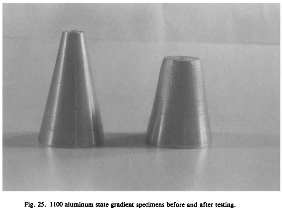
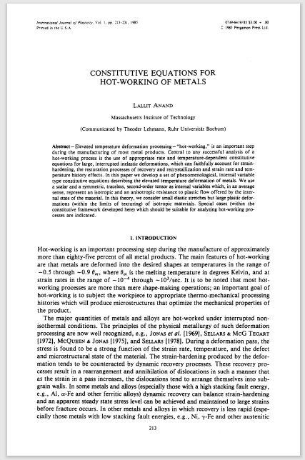
Constitutive Equations for Hot-Working of Metals
Author: Lallit Anand (1985)
One of the foundational papers in thermodynamically consistent viscoplasticity modeling—especially significant in the context of metals subjected to large strains and high temperatures.
Case Study: Wang (2001) Apply to Solder
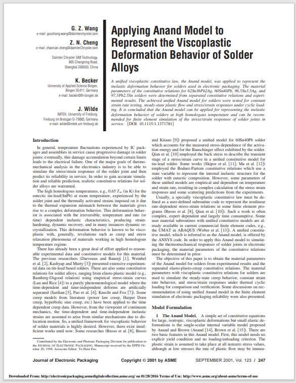
Source: Wang, C. H. (2001). “A Unified Creep–Plasticity Model for Solder Alloys.”
DOI: 10.1115/1.1371781
DOI: 10.1115/1.1371781
Why Wang's Paper Matters
- Applies Anand’s unified viscoplastic framework to model solder behavior.
- Anand's model can be reduced and fitted from experiments.
- transition the theory into engineering-scale implementation.
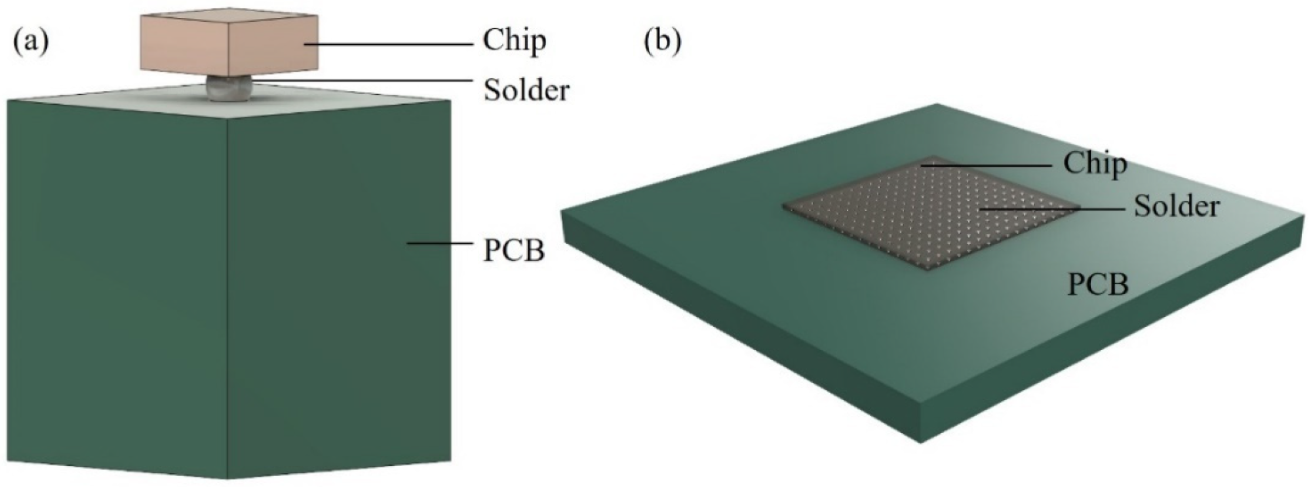
- Targets solder joints in microelectronic packages (chip on PCB, soldered connections).
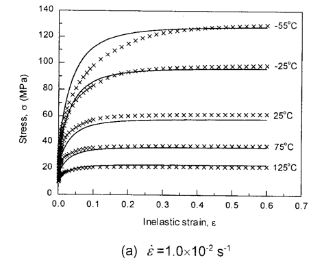
Comparing Anand Model Predictions at Two Strain Rates
Observed Behavior
- Top Graph (a): \( \dot{\varepsilon} = 10^{-2} \, \text{s}^{-1} \)
- High strain rate → higher stress
- Recovery negligible → pronounced hardening
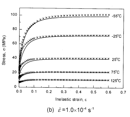
- Bottom Graph (b): \( \dot{\varepsilon} = 10^{-4} \, \text{s}^{-1} \)
- Lower strain rate → lower stress at same strain
- Recovery and creep effects more significant
Model Accuracy: Lines = model prediction, X = experimental data
Key Insights from Wang (2001)
- “At lower strain rates, recovery dominates… the stress levels off early.”
- “At high strain rates, hardening dominates, and the stress grows continuously.”
Anand’s model smoothly captures strain-rate and temperature dependence of solder materials.
Main Equations of Wang’s Anand-Type Viscoplastic Model
Flow Rule (Plastic Strain Rate)
- \[ \dot{\varepsilon}^p = A \exp\left( -\frac{Q}{RT} \right) \left[ \sinh\left( \frac{j \sigma}{s} \right) \right]^{1/m} \]
- Plastic strain rate increases with stress and temperature.
- No explicit yield surface; flow occurs at all nonzero stresses.
Deformation Resistance Saturation \( s^* \)
- \[ s^* = \hat{s} \left( \frac{\dot{\varepsilon}^p}{A} \exp\left( \frac{Q}{RT} \right) \right)^n \]
- Defines the steady-state value that \( s \) evolves toward.
- Depends on strain rate and temperature.
Evolution of Deformation Resistance \( s \)
- \[ \dot{s} = h_0 \left| 1 - \frac{s}{s^*} \right|^a \, \text{sign}\left(1 - \frac{s}{s^*}\right) \dot{\varepsilon}^p \]
- Describes dynamic hardening and softening of the material.
- \( s \) evolves depending on proximity to \( s^* \) and flow activity.
Note: Constants \( A, Q, m, j, h_0, \hat{s}, n, a \) are material-specific and fitted to experimental creep/strain rate data.
Anand Viscoplasticity Constants for 60Sn40Pb
Image Reference
Values are from correspond to 60Sn40Pb solder parameters used in Anand's model:
- \( S_0 \): Initial deformation resistance
- \( Q/R \): Activation energy over gas constant
- \( A \): Pre-exponential factor for flow rate
- \( \xi \): Multiplier of stress inside sinh
- \( m \): Strain rate sensitivity of stress
- \( h_0 \): Hardening/softening constant
- \( \hat{s} \): Coefficient for saturation stress
- \( n \): Strain rate sensitivity of saturation
- \( a \): Strain rate sensitivity of hardening or softening
Numerical Values
- \( S_0 = 5.633 \times 10^7 \) Pa
- \( Q/R = 10830 \) K
- \( A = 1.49 \times 10^7 \) s\(^{-1}\)
- \( \xi = 11 \)
- \( m = 0.303 \)
- \( h_0 = 2.6408 \times 10^9 \) Pa
- \( \hat{s} = 8.042 \times 10^7 \) Pa
- \( n = 0.0231 \)
- \( a = 1.34 \)
These constants match Wang's paper for modeling 60Sn40Pb viscoplasticity.
Forward Euler Explicit time integration scheme Pseudocode
Initialization
- Material constants: \( A, Q/R, j, m, h_0, \hat{s}, n, a, E \)
- Strain rate: \( \dot{\varepsilon} \)
- Temperature set: \( \{ T_i \} \)
- Set: \( \varepsilon^p(0) = 0, \quad s(0) = \hat{s} \)
Time Evolution Loop
- \( \varepsilon_{\text{total}}(t) = \dot{\varepsilon} t \)
- \( \sigma_{\text{trial}} = E (\varepsilon_{\text{total}} - \varepsilon^p) \)
- Compute \( x = \frac{j \sigma}{s} \)
- Approximate \( \sinh(x) \) (linearize if \( |x| \ll 1 \))
- \( \dot{\varepsilon}^p = A e^{-Q/RT} (\sinh(x))^{1/m} \)
Plastic Flow & Resistance Evolution
- \( s^* = \hat{s} \left( \frac{\dot{\varepsilon}^p}{A} e^{Q/RT} \right)^n \)
- \( \dot{s} = h_0 \left| 1 - \frac{s}{s^*} \right|^a \text{sign}\left(1 - \frac{s}{s^*}\right) \dot{\varepsilon}^p \)
- Update: \( \varepsilon^p(t+\Delta t) = \varepsilon^p(t) + \dot{\varepsilon}^p \Delta t \)
- Update: \( s(t+\Delta t) = s(t) + \dot{s} \Delta t \)
- Record \( (\varepsilon_{\text{total}}, \sigma_{\text{trial}}) \)
Termination
- Stop when \( \varepsilon_{\text{total}} \geq \varepsilon_{\text{max}} \)
- Plot \( \sigma \) vs \( \varepsilon \) for all \( T_i \)
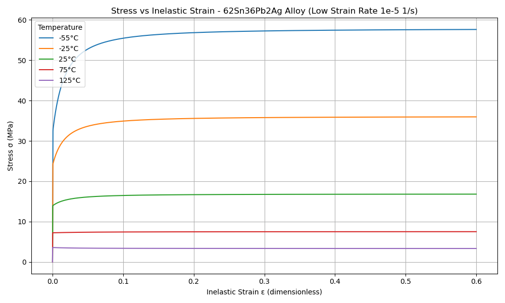
Forward Euler Scheme for Anand Model
import numpy as np
import matplotlib.pyplot as plt
from scipy.integrate import solve_ivp

# Material constants for 62Sn36Pb2Ag solder alloy
A = 2.24e8       # 1/s
Q_R = 11200      # K
j = 13           # dimensionless
m = 0.21         # dimensionless
h0 = 1.62e10     # Pa
s0 = 8.47e7      # Pa
s_hat = 8.47e7   # Pa
n = 0.0277       # dimensionless
a = 1.7          # dimensionless
E = 5.2e10       # Pa (Elastic modulus)

# Temperatures in Kelvin
T_C = [-55, -25, 25, 75, 125]
T_list = [T + 273.15 for T in T_C]

# Simulation parameters
strain_rate = 1e-5  # 1/s
eps_total_max = 0.6
t_max = eps_total_max / strain_rate
time_steps = 10000
t_eval = np.linspace(0, t_max, time_steps)

# Define the ODE system
def system(t, y, T):
    ep_p, s = y
    eps_total = strain_rate * t
    sigma_trial = E * (eps_total - ep_p)
    x = j * sigma_trial / s

    if np.abs(x) < 0.01:
        sinh_x = x
    else:
        sinh_x = np.sinh(np.clip(x, -30, 30))

    sinh_x = np.maximum(sinh_x, 1e-12)
    dep_p = A * np.exp(-Q_R / T) * sinh_x**(1/m)

    s_star = s_hat * (dep_p / A * np.exp(Q_R / T))**n
    ds = h0 * np.abs(1 - s/s_star)**a * np.sign(1 - s/s_star) * dep_p

    return [dep_p, ds]

# Plotting
plt.figure(figsize=(9,6))

for T in T_list:
    sol = solve_ivp(system, [0, t_max], [0, s0], args=(T,), t_eval=t_eval, method='Radau', rtol=1e-6, atol=1e-9)
    eps_total = strain_rate * sol.t
    sigma = E * (eps_total - sol.y[0])

    label = f"{int(T-273.15)}°C"
    plt.plot(eps_total, sigma/1e6, label=label)

plt.xlabel("Inelastic Strain ε (dimensionless)")
plt.ylabel("Stress σ (MPa)")
plt.title("Stress vs Inelastic Strain - 62Sn36Pb2Ag Alloy (Low Strain Rate 1e-5 1/s)")
plt.grid(True)
plt.legend(title="Temperature")
plt.xlim([0, 0.6])
plt.ylim([0, 65])
plt.tight_layout()
plt.show()
Strain rate sensitivity of stress m
- As \( m \to 0 \), rate insensitive (yield)
- As \( m \to 1 \), small stress change causes big change in strain rate
Flow rule
Tensorial Flow Rule (directional form)
\[
\mathbf{D}^p = \dot{\epsilon}^p \left( \frac{3}{2} \frac{\mathbf{T}'}{\bar{\sigma}} \right)
\]
Equivalent Stress Definition
\[
\bar{\sigma} = \sqrt{\frac{3}{2} \mathbf{T}':\mathbf{T}'}
\]
Plastic Strain Rate (magnitude form)
\[
\dot{\epsilon}^p = A \exp\left( -\frac{Q}{R\theta} \right) \left[ \sinh\left( \xi \frac{\bar{\sigma}}{s} \right) \right]^{1/m}
\]
Full Flow Rule with Hyperbolic Sine
\[
\mathbf{D}^p = A \exp\left( -\frac{Q}{R\theta} \right) \left[ \sinh\left( \xi \frac{\bar{\sigma}}{s} \right) \right]^{1/m} \left( \frac{3}{2} \frac{\mathbf{T}'}{\bar{\sigma}} \right),
\]
\[ = \dot{\gamma}^p \left( \frac{\widetilde{\mathbf{T}}'}{2 \bar{\tau}} \right), \quad \bar{\tau} = \left\{ \frac{1}{2} \text{tr}(\widetilde{\mathbf{T}}'^2) \right\}^{1/2} \]
\[ = \dot{\gamma}^p \left( \frac{\widetilde{\mathbf{T}}'}{2 \bar{\tau}} \right), \quad \bar{\tau} = \left\{ \frac{1}{2} \text{tr}(\widetilde{\mathbf{T}}'^2) \right\}^{1/2} \]
Summary:
- Direction given by \( \mathbf{T}' \).
- Magnitude determined by hyperbolic sine based on \( \bar{\sigma}/s \).
- \( \bar{\tau} \) represents the effective shear stress computed from deviatoric stress.
- \(\bar{\sigma} = \sqrt{\frac{3}{2} \mathbf{T'} : \mathbf{T'} }\) is the von Mises Equivalent stress, but is formally defined without yield point
- Full flow = direction × magnitude.
Evolution Equation for the Stress
Stress Evolution Equation (Rate form of Hooke's Law)
\[
\overset{\nabla}{\mathbf{T}} = \mathbb{L} \left[ \mathbf{D} - \mathbf{D}^p \right] - \boldsymbol{\Pi} \dot{\theta}
\]
(rate-form Hooke’s law for finite deformation plasticity, with frame-indifference enforced through the Jaumann rate.)
Jaumann Rate Definition
\[
\overset{\nabla}{\mathbf{T}} = \dot{\mathbf{T}} - \mathbf{W}\mathbf{T} + \mathbf{T}\mathbf{W}
\]
Material Tensors and Operators
- \( \mathbb{L} = 2\mu \mathbf{I} + \left( \kappa - \frac{2}{3}\mu \right) \mathbf{1} \otimes \mathbf{1} \) — isotropic elasticity tensor
- \(\mathbb{L}\mathbf{D} \) represents how instantaneous strain rates generate stresses according to the elastic material's stiffness properties.
- \( \mu = \mu(\theta) \), \( \kappa = \kappa(\theta) \) — temperature-dependent moduli
- \( \boldsymbol{\Pi} = (3\alpha \kappa) \mathbf{1} \) — stress-temperature coupling
- \( \alpha = \alpha(\theta) \) — thermal expansion coefficient
- \( \mathbf{D} = \text{sym}(\nabla \mathbf{v}) \) — stretching tensor
- \( \mathbf{W} = \text{skew}(\nabla \mathbf{v}) \) — spin tensor
- \( \mathbf{I} \) = fourth-order identity tensor
- \( \mathbf{1} \) = second-order identity tensor
Summary:
- Stress rate follows Jaumann derivative to ensure frame indifference.
- Elastic response governed by isotropic fourth-order tensor \( \mathbb{L} \).
- Thermal expansion introduces additional stress through \( \boldsymbol{\Pi} \dot{\theta} \).
Stress Evolution and Thermal Effects
Stress Evolution and Thermal Effects
In the stress evolution equation,
\[
\overset{\nabla}{\mathbf{T}} = \mathbb{L} \left[ \mathbf{D} - \mathbf{D}^p \right] - \boldsymbol{\Pi} \dot{\theta},
\]
the term \( \boldsymbol{\Pi} \dot{\theta} \) represents the stress change that would occur due to pure thermal expansion alone, without any mechanical loading.
Why Subtract the Thermal Term?
- Thermal expansion creates strain even without external forces.
- Without subtracting \( \boldsymbol{\Pi} \dot{\theta} \), the model would falsely attribute thermal strain as mechanical stress.
- Subtracting isolates the true mechanical response from thermal effects.
Summary:
- Thermal expansion induces strain without force.
- Subtracting \( \boldsymbol{\Pi} \dot{\theta} \) ensures only mechanical strains generate stresses.
- This keeps the constitutive model physically accurate during heating and cooling.
Relaxed (Intermediate) Configuration
Context for the Relaxed Configuration
- The relaxed configuration represents the material after removing plastic deformations but before applying new elastic deformations.
- It is introduced to separate permanent plastic effects from recoverable elastic effects.
- All thermodynamic potentials, internal variables, and evolution laws are defined relative to this frame.
- The relaxed state provides a clean, natural reference for measuring elastic strain \( E^e \) and computing dissipation.
What Happens in the Relaxed Configuration?
- The elastic deformation gradient \( F^e \) is measured from the relaxed state to the current deformed state.
- Elastic strain measures like \( C^e \) and \( E^e \) are defined in this configuration.
- The Kirchhoff stress \( \widetilde{\mathbf{T}} \) is naturally associated with the relaxed volume.
- Plastic flow is accounted for separately through the plastic velocity gradient \( \mathbf{L}^p \).
Summary:
- The relaxed configuration isolates elastic responses cleanly, enabling proper definition of thermodynamics and plastic evolution laws.
Relaxed Configuration Constituative Laws
Kinematics in the Relaxed Configuration
- Elastic deformation gradient:
\[ F = F^e F^p \quad \Rightarrow \quad F^e = F F^{p-1} \]
- Elastic right Cauchy-Green tensor:
\[ C^e = F^{eT} F^e \]
- Elastic Green–Lagrange strain tensor:
\[ E^e = \frac{1}{2} (C^e - I) \]
Stress and Power Quantities
- Kirchhoff stress (weighted Cauchy stress):
\[ \widetilde{\mathbf{T}} = (\det F) \mathbf{T} \]
- Stress power split:
\[ \dot{\omega} = \dot{\omega}^e + \dot{\omega}^p \] \[ \dot{\omega}^e = \widetilde{\mathbf{T}} : \dot{E}^e \quad , \quad \dot{\omega}^p = (C^e \widetilde{\mathbf{T}}) : \mathbf{L}^p \]
Summary:
- Elastic kinematics and stress measures are formulated relative to the relaxed configuration, cleanly separating plastic and elastic contributions.
- Stress Power Split allows Anand to cleanly isolate plastic dissipation from elastic storage.
- Green-Lagrange strain tensor \(E^e\) is used because it symmetrically captures nonlinear elastic strain relative to the relaxed configuration
- The right Cauchy-Green tensor \(C^e = F^{e^T}F^e\) is required as an intermediate to compute \(E^e\) from the elastic deformation gradient \(F^e\) without referencing spatial coordinates
Dissipation Separation: Elastic vs Plastic in Anand’s Model
Thermodynamic Separation
- Start with Total Dissipation:
\[ \mathcal{D} = \dot{\omega} - \dot{\psi} \geq 0 \] where \(\dot{\omega} = \widehat{\mathbf{T}} : \dot{\mathbf{E}}^e + (\mathbf{C}^e \widehat{\mathbf{T}}) : \mathbf{L}^p\) - Split Stress Power:
\[ \dot{\omega} = \dot{\omega}^e + \dot{\omega}^p \] with:- \( \dot{\omega}^e = \widehat{\mathbf{T}} : \dot{\mathbf{E}}^e \)
- \( \dot{\omega}^p = (\mathbf{C}^e \widehat{\mathbf{T}}) : \mathbf{L}^p \)
- Group Terms with \( \dot{\psi} \):
\[ (\dot{\omega}^e - \dot{\psi}) + \dot{\omega}^p \geq 0 \] - Apply Elastic Energy Consistency:
\[ \dot{\omega}^e - \dot{\psi} = 0 \quad \Rightarrow \quad \dot{\omega}^p \geq 0 \]
Key Physical Insights
- Elastic deformations are recoverable and do not cause entropy production.
- All dissipation stems from the plastic flow: \(\dot{\omega}^p\).
- Plastic work increases entropy and governs viscoplastic evolution.
Summary:
The stress power split ensures that the second law is satisfied by assigning dissipation solely to irreversible processes.
The stress power split ensures that the second law is satisfied by assigning dissipation solely to irreversible processes.
Reference Configuration
Framework in the Reference Configuration
- The free energy \( \psi \) is defined relative to the reference configuration.
- State variables like \( E^e, \theta, \bar{g}, \mathbf{\bar{B}}, s \) are used as arguments of \( \psi \).
- Stress is expressed using the second Piola–Kirchhoff tensor \( \mathbf{S} \).
- Dissipation inequality, stress–strain relations, and evolution laws are all written in reference variables.
- Mass density \( \rho_0 \) from the reference configuration normalizes all terms.
Key Equations in the Reference Frame
- Free energy:
\[ \boxed{ \psi = \psi(E^e, \theta, \bar{g}, \mathbf{\bar{B}}, s) } \]
- Dissipation inequality:
\[ \boxed{ \dot{\psi} + \eta \dot{\theta} - \rho_0^{-1} \mathbf{S} : \dot{E} + (\rho_0 \theta)^{-1} \mathbf{q}_0 \cdot \mathbf{g}_0 \leq 0 } \]
- Constitutive relation:
\[ \boxed{ \mathbf{S} = \rho_0 \frac{\partial \psi}{\partial E^e} } \]
Summary:
- In the reference configuration, all energy storage, stress updates, and internal variable evolution are formulated with reference-frame quantities for consistency and objectivity.
Thermodynamics
Thermodynamic Quantities
- Free energy density:
\[ \boxed{ \psi = \epsilon - \theta \eta } \]
- Reduced dissipation inequality:
\[ \boxed{ \dot{\psi} + \eta \dot{\theta} - \rho^{-1} \mathbf{T} : \mathbf{L} + (\rho \theta)^{-1} \mathbf{q} \cdot \mathbf{g} \leq 0 } \]
- State variables: \[ \{ E^e, \theta, \bar{g}, \mathbf{\bar{B}}, s \} \] with \( E^e \) as elastic strain and \( s \) as internal resistance.
Stress Power and Kirchhoff Stress
- Stress power per relaxed volume:
\[ \boxed{ \dot{\omega} = \left( \frac{\rho_0}{\rho} \right) \mathbf{T} : \mathbf{L} } \]
- Weighted Cauchy (Kirchhoff) stress:
\[ \boxed{ \mathbf{\widetilde{T}} = (\det F) \mathbf{T} } \quad \text{or} \quad \boxed{ \mathbf{\widetilde{T}} = \left( \frac{\rho_0}{\rho} \right) \mathbf{T} } \]
- Decomposition of stress power:
\[ \boxed{ \dot{\omega} = \dot{\omega}^e + \dot{\omega}^p } \] \[ \dot{\omega}^e = \mathbf{\widetilde{T}} : \dot{E}^e, \quad \dot{\omega}^p = (C^e \mathbf{\widetilde{T}}) : \mathbf{L}^p \]
Summary:
- Free energy and dissipation govern thermodynamic consistency.
- Stress power naturally splits into elastic and plastic parts.
- Kirchhoff stress simplifies stress evolution accounting for volume changes.